Regression Language Models: Predicting Anything from Raw Text
Two recent papers from Google ask a simple question: what happens if you treat regression as a next-token prediction problem? Feed a raw text string into an encoder-decoder, decode the output scalar digit by digit, and train using cross-entropy loss. The result, which they call a Regression Language Model (RLM), achieves 0.99 rank correlation on Google's Borg compute cluster and outperforms graph neural networks on neural architecture search benchmarks. We think the implications for ML model search are significant.
The Feature Engineering Problem
Traditional regression requires compressing the input state into a fixed-length vector in . For structured, tabular data this is straightforward.
For real system data, it is not. Take Borg, Google's compute cluster scheduler. Predicting its efficiency metric requires ingesting cluster configuration, hardware distributions, scheduler hyperparameters, and job-on-machine profiling results. The job profiling feature alone averages 268,157 characters per input. Features have arbitrary cardinalities, deep nesting, and change whenever hardware changes. Every time a new machine class is introduced, the feature schema breaks and the training data produced under the old schema becomes invalid.
The same problem appears in code. Predicting the memory footprint or execution latency of a program requires understanding its structure. Representing a computation graph as a fixed-length vector requires choosing a graph encoding. When the set of possible operations changes, the encoding needs to be redesigned from scratch.
There's a formal argument for why this is the case. Define the epistemic uncertainty induced by a featurization as:
where are the equivalence classes of inputs that cannot distinguish. If collapses two distinct states and to the same representation, no regressor can do better than predicting their average outcome. The expected squared error of any pointwise regressor is lower bounded by:
This quantity provides a hard lower bound on the MSE achievable by any model using featurization . A tabular featurization that drops nested or variable-length fields merges many distinct states into the same equivalence class , each producing different outcomes . The within-class variance is high, and no regressor can beat it. A text representation that preserves all available information makes each equivalence class a singleton, collapsing the bound to pure aleatoric uncertainty: the irreducible noise in given the full state of the world.
The RLM Approach
The core method is straightforward. Represent the input as a string (YAML, source code, ONNX IR, or any structured text). Then feed it to an encoder and decode the output digit-by-digit using a custom P10 tokenization in which a float like is represented as the token sequence <+><7><2><5><E-1>, encoding sign, mantissa digits, and exponent. Train with standard next-token cross-entropy over the response tokens.
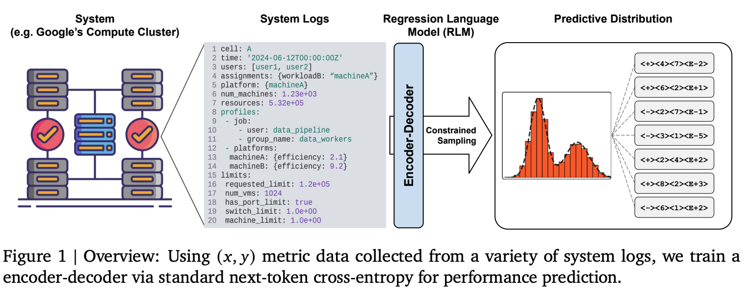 Figure 1 (Borg paper): The RLM reads raw system log strings through an encoder and decodes numeric predictions token by token. The output is a full density , not just a point estimate.
Several design choices here are worth highlighting, because they go against common practice:
No language pretraining (for the Borg paper). The model for system performance prediction is trained from random initialization purely on pairs. Language pretraining is not needed when the task is regression over structured tokens rather than natural language generation. The model only needs to learn correlations between structured input tokens and numeric outputs.
Encoder-decoder over decoder-only. Modern LLMs are almost universally decoder-only. But for regression over complex inputs, dedicated encoder layers matter. In ablations, encoder-decoder architectures substantially outperform decoder-only ones at equal parameter count, even when the decoder-only model uses bidirectional attention on the input. The hypothesis is that decoder information pathways are insufficient for processing complex, high-dimensional inputs .
Cross-entropy over MSE. Training with cross-entropy on digit tokens is scale-agnostic. MSE loss is sensitive to -value scale, which causes instability when training a single model on tasks with very different output ranges. Cross-entropy avoids this and makes multi-task training natural.
Context-free. The model maps a single to a single , aggregating i.i.d. samples , rather than conditioning on in-context pairs. This maximizes the sequence budget for the input representation and allows unlimited training data to be absorbed into weights rather than being constrained by a finite context buffer.
Results on Google's Borg Cluster
The Borg paper applies this to predicting MIPS per GCU, a productivity metric for Google's compute cluster. A single simulation of the cluster's digital twin takes between 1 and 18 hours. The RLM replaces this with negligible inference time.
A 60M parameter encoder-decoder, pretrained on approximately 1M data points from 8 cluster tasks, achieves 0.86 Spearman rank correlation in-distribution. Fine-tuned on 512 examples from a completely new, unseen cluster, it matches this performance out-of-distribution. A randomly initialized model given the same 512 examples cannot.
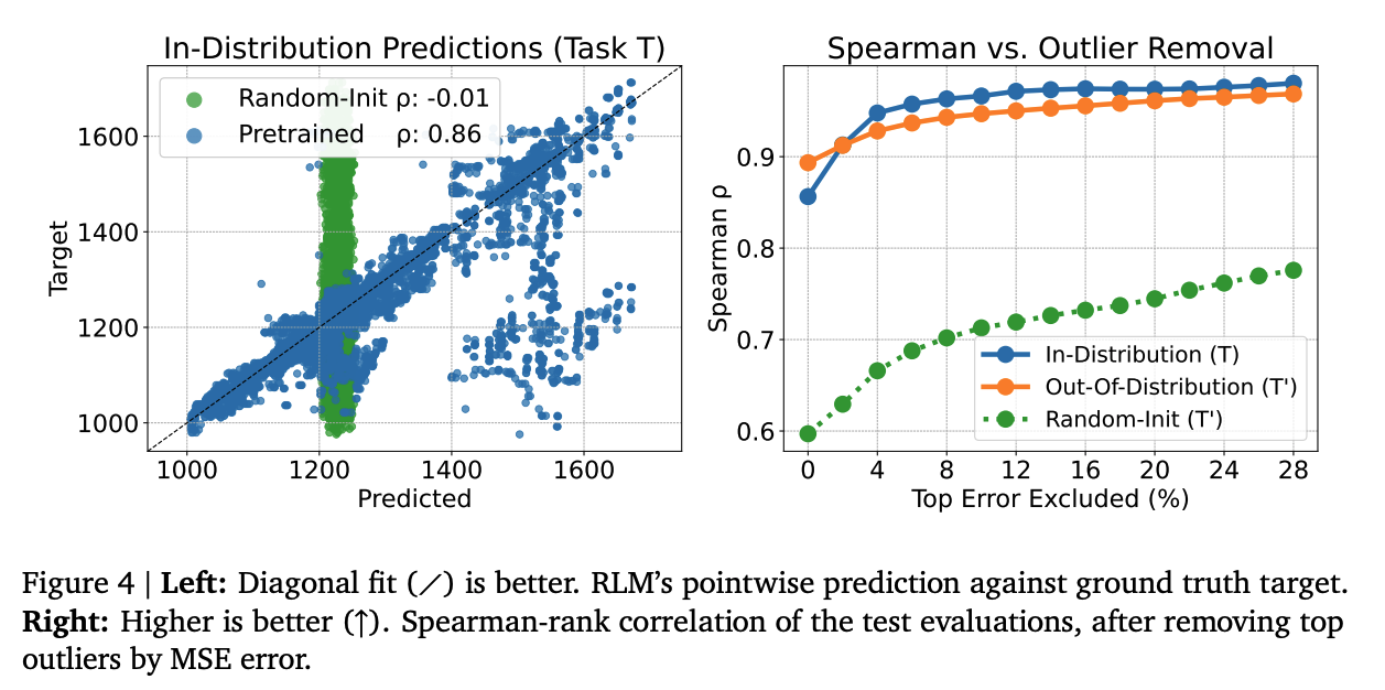 Figure 4 (Borg paper): Left: pretrained RLM predictions against ground truth () vs. random initialization (). Right: Spearman rank correlation as a function of outliers removed, showing the pretrained model (blue/orange) consistently dominates random initialization (green).
Across a broader evaluation over 40 cells, the majority of tasks reach Spearman rank above 0.93, with the best at 0.99. The few-shot transfer result is especially striking: with more pretraining tasks, the model generalizes to unseen clusters from very few examples, while a model pretrained on only one task barely improves with fine-tuning data.
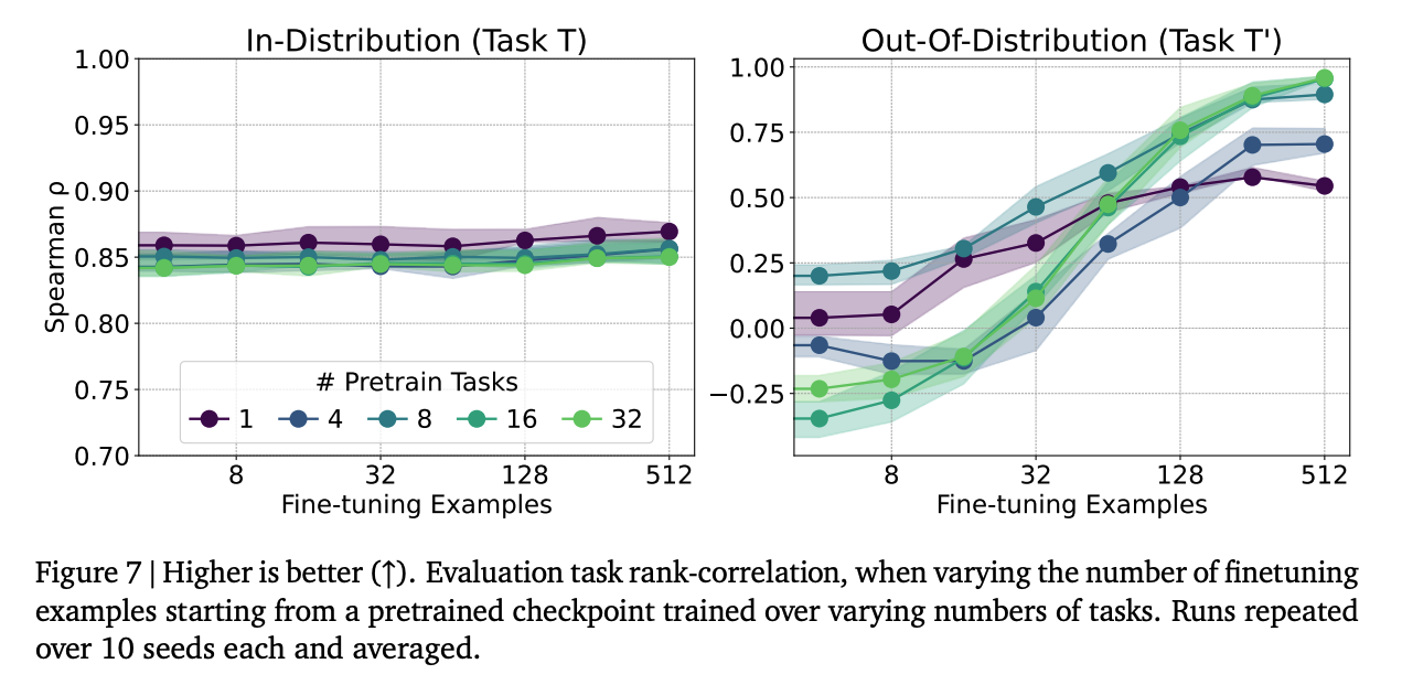 Figure 7 (Borg paper): Out-of-distribution rank correlation as a function of fine-tuning examples, for models pretrained on 1 to 32 tasks. More pretraining diversity leads to substantially better transfer to unseen clusters.
The output is also a full density . Prediction variance correlates with residual error (Spearman ), and the model naturally expresses bimodality on noisy tasks without being explicitly trained to do so.
RLMs for Code
The second paper extends the same method to code. A 300M parameter RLM initialized from T5Gemma is trained jointly on memory prediction across 24 programming languages (CodeNet), latency prediction for Triton GPU kernels (KernelBook), and peak memory prediction on competitive programming submissions (APPS). The same model also ingests ONNX representations of neural network architectures for neural architecture search.
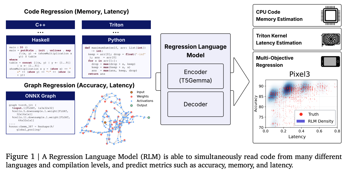 Figure 1 (Code paper): A single RLM simultaneously reads code from many different languages and compilation levels, predicting metrics including accuracy, memory, and latency.
On APPS Leetcode peak memory prediction, the RLM achieves Spearman rank 0.93. On CodeNet, it achieves above 0.6 on C++ and Python, and non-trivial results across more obscure languages like Lua, Haskell, and OCaml. Triton kernel latency reaches 0.52.
Beating GNNs at Their Own Game
For NAS, the RLM reads raw ONNX strings and predicts architecture accuracy on CIFAR-10. This is the setting where you would most expect a text-based model to lose: graph neural networks are specifically designed to operate over computation graphs, with inductive biases for connectivity patterns and node features that a text model has to infer from a linearized string. Despite this, the RLM achieves the highest average Kendall- of 0.46 across five classic NAS design spaces, beating GNNs and matching the previous state of the art (FLAN). Kendall- measures rank correlation between predicted and true accuracy scores: how well the model orders architectures by quality, which is what matters in search. FLAN reaches its performance by supplementing the architecture representation with zero-cost proxies: cheap statistics computed at initialization, before any training, that correlate with final accuracy. The RLM uses none of these; it predicts from the ONNX string alone.
| Method | Average Kendall- |
|---|---|
| MLP (Adjacency) | 0.052 |
| Arch2Vec | 0.212 |
| CATE | 0.238 |
| GNN | 0.429 |
| FLAN (previous SoTA) | 0.459 |
| RLM (ours) | 0.461 |
Do You Even Need a Regression Head?
A common assumption is that using a language model for regression requires attaching an explicit regression head: an MLP on top of a pooled encoder state, trained with MSE loss. The code paper includes a clean ablation that refutes this.
The comparison uses the same total layer count for fairness: an encoder-decoder (2 layers each) trained with cross-entropy against an encoder-only model (4 layers) with an MLP regression head trained with MSE. They are evaluated on three NAS spaces with very different -value ranges: roughly - for NASBench-101, for SNAS, and for the OFA family.
This range variation is the crux. MSE loss is sensitive to scale, so a head trained on NASBench-101 accuracy is not directly comparable to one trained on OFA accuracy. The paper evaluates two variants: an unnormalized head and a normalized head where -values are linearly scaled to per dataset.
| Head | Spearman |
|---|---|
| Regression head (unnormalized) | 0.478 |
| Regression head (normalized) | 0.717 |
| Decoder head (cross-entropy) | 0.800 |
Normalization helps the regression head substantially, going from 0.478 to 0.717. But the decoder head still wins at 0.800, and crucially it requires no normalization at all. The P10 tokenization represents any float regardless of scale, so a single model can train on NASBench-101 and OFA simultaneously without any per-dataset preprocessing. This is a meaningful practical advantage when building a unified surrogate across many search spaces.
The key is the ONNX representation. ONNX is a universal intermediate representation for computation graphs that encodes the full auto-differentiation graph: all operations, shapes, and connectivity. It is also the standard format used in ML compiler optimization pipelines, which means the same RLM trained for NAS could plausibly transfer to compiler optimization tasks without retraining.
Multi-Hardware Latency Prediction in One Model
Because the decoder generates outputs sequentially, predicting multiple metrics is straightforward: decode accuracy, then latency on Pixel3, then Eyeriss (ASIC), then Intel CPU, then Nvidia GPU, each conditioned on the previous outputs. Formally, the joint distribution factors as:
This matters because the objectives are not independent. A very low-latency architecture is probably too small to achieve high accuracy. Knowing the predicted latency should sharpen the prediction of accuracy. Parallel regression heads cannot do this: when each objective is read off the same pooled embedding independently, and are conditionally independent given :
The autoregressive decoder has no such constraint. It can learn that a predicted low-latency token sequence should shift the distribution over subsequent accuracy tokens downward. This is the architecturally correct way to model correlated objectives, and it comes for free from the sequential decoding structure.
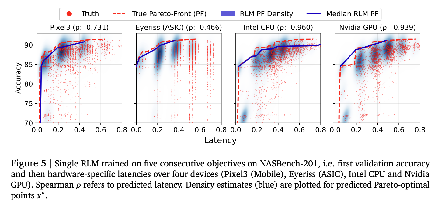 Figure 5 (Code paper): A single RLM trained on five consecutive objectives (validation accuracy then hardware latencies on Pixel3, Eyeriss, Intel CPU, Nvidia GPU). The density estimates (blue) for predicted Pareto-optimal architectures correctly tilt to reflect the positive correlation between accuracy and latency.
Language pretraining does matter for code, unlike for system logs. Initializing from T5Gemma leads to faster convergence and better final performance than training from scratch, presumably because code shares structural patterns with natural language. A custom ONNX-aware tokenizer (8K tokens vs T5's 32K) also helps substantially, reducing token counts and allowing longer graphs to fit within the sequence budget.
The Application We Find Most Interesting
The most immediate practical implication of this work is for ML model search. Any system that proposes candidate architectures or configurations needs to evaluate them. Training a model to convergence is expensive. Zero-cost proxies are cheap but imprecise. Simulation-based methods (like Borg's digital twin) are accurate but slow.
An RLM offers a middle path: a learned surrogate that is fast at inference time, accurate enough to rank candidates reliably, and adaptable to new search spaces with a small number of labeled examples. This is exactly the regime where a system like AlphaEvolve operates. AlphaEvolve maintains a population of candidate programs, uses LLMs to propose mutations, and needs to score candidates quickly to decide which ones to keep. Plugging an RLM in as the evaluator replaces expensive training runs with a forward pass.
The code RLM paper shows this is already viable for NAS. The next step is extending it to the broader class of ML experiments: predicting the downstream accuracy of a pretraining run from its configuration, or scoring a reward model from its training setup. Whether the RLM can generalize reliably enough in these settings is an open question, but the results on out-of-distribution cluster tasks suggest that with enough pretraining diversity, transfer is achievable.
Takeaways
Both papers make the same core argument from different angles: when your input is complex, nested, and hard to featurize, the right move is to not featurize it at all. Represent it as text, train an encoder-decoder with cross-entropy, and let the model learn the relevant structure from data.
The practical payoff is real. A 60M parameter model replaces 1 to 18 hour simulations for cluster optimization. A 300M parameter model predicts code memory and latency across 24 programming languages without any language-specific feature engineering.
For anyone building systems that require fast, repeated evaluation of complex configurations, this is a straightforward technique worth adopting.
Papers:
Akhauri et al. (2025). Performance Prediction for Large Systems via Text-to-Text Regression. Google / Cornell. Code
Akhauri and Song et al. (2025). Regression Language Models for Code. Google / Cornell. Code · Dataset